What are the error bars on your faith?

by Tom Crawford

6/23/2008

(previous)
(back to index)

• How confident are you in what you believe?
• What are the error bars or limits of uncertainty to your faith?
• What is the probability that you believe something wrong?

All these questions are related.  Are you certain that what you believe is true?  What is the probability that you are wrong?  How would you know or quantify it?  At this point, I’m going to be generic.  In talking about faith, I want you to know that I could be talking about your faith in God, in a god, or that there is no god; your faith in evolution, the Big Bang, or a law of physics; your faith in the chair in which you are sitting or the bridge that you are driving across; or your faith in anything else that you believe to be true.  Things that we believe to be true always have some level of uncertainty.  The level of uncertainty we have in our faith is inversely proportional to our true knowledge of the thing in which we are placing our faith.

In science and engineering, we usually quantify how much faith we can reasonably place in an observation, a measurement, or a set of data.  We do this by specifying the level of uncertainty or the error bars of our measurement or data set.  In other words, we are very confident that the true value of what we are trying to measure falls within a narrow range of values.  So how do we measure how certain or uncertain we are in a particular measurement or observation?  Following are a couple of examples:

Faith and its relationship with knowledge. In my previous blogs I discussed how faith and knowledge are related - not inversely as Schopenhauer stated - but proportionally. The more true knowledge I have about a subject or object, the more faith I can reasonably place in that subject or object. This follows from the definition of faith, both in English and in the Greek (the language in which the New Testament was written). It follows then, that the error bars on my faith in something (or the limits of uncertainty to my faith) are proportional to the uncertainty or the error bars in my knowledge of the truth about the thing in which I am placing my faith.

How do I quantify limits of uncertainty?  What are error bars?  What is my probability of being right or wrong?

Example 1 – a political poll

The USA is currently in a presidential election season (summer 2008).  We hear a lot about political polls.  A good poll is accompanied by a level of uncertainty or a set of error bars.  For example, a poll might look like:

• Candidate A             46%
• Candidate B             43%
• Undecided                11%
• Margin of error        ± 3%

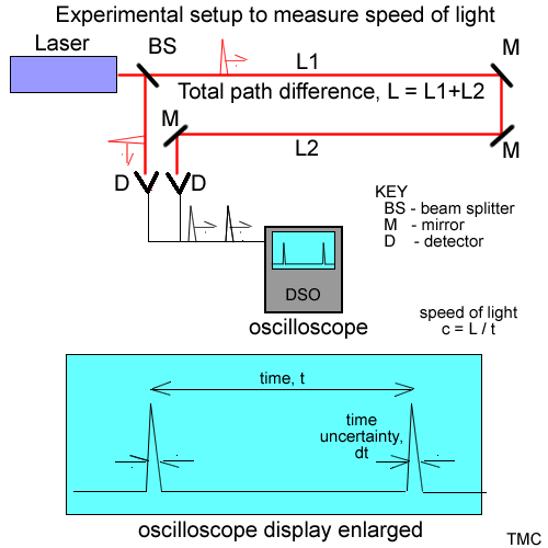
The margin of error or level of uncertainty in the poll (the poll's error bars) is dependent on the number of people the pollsters survey, and on how well the people they surveyed represent the general voting population.  The plus or minus ( ±) value given for the margin of error is a standard deviation.  If the polling model is a good representative model of the voting population, then the standard deviation is simply the square root of the number of people surveyed divided by the number of people surveyed ( √N / N ).  Using the standard deviation means that the pollsters are confident that if the election were held today, the actual results would have a 68% chance of falling somewhere within the poll numbers plus or minus the margin of error.  They have stated how much faith they can place in that poll.

Example 2 – a lab experiment measuring the speed of light

Suppose we are in a physics lab and are doing an experiment to measure the speed of light.  (No – you have not died and woken up in hell - that's more like an English literature class.  LOL.)  To do this, we set up the experiment shown in the following schematic diagram.

Experimental schematic on measuring the speed of light. A pulsed laser is our light source.  It generates short pulses of only a few nanoseconds in duration.  We pass these laser pulses through a beam splitter (BS) producing two pulsed beams - a reference beam and a beam which bounces off of some distant mirrors (M) somewhere across campus.  Both the reference beam and the experiment beam are then detected using photo diodes or some other form of optical detectors (D).  The detection of both the reference pulse and the experiment pulse form electrical current pulses which are then detected by a digital storage oscilloscope (DSO).  The DSO allows us to measure the time between the reference pulse and the experiment pulse.  If we know the time between the two pulses, and we know how much further the experiment pulse traveled than the reference pulse, we can calculate the speed of light by dividing the distance by the time.

After setting up the experiment we shoot one laser pulse through the experimental setup, measure the time between the reference and experimental pulses, and calculate the speed of light.  We get a value of 3.1 * 10⁸ meters per second.  We write up our experiment and hand our lab report to the professor, who promptly asks us, “Do you believe your answer?  How much faith can you put into your value of the speed of light?”  We tell him, “We set up the experiment and it worked.  We obviously have shown that light travels at a finite speed.”  He then asks, “Would you stake your life on this value?  If we were to program this value into the ring laser gyroscopes and other guidance equipment on the next space shuttle, would you fly on that shuttle?”  We don’t have an answer - so back to the lab.  At the present time, we do not know how much confidence or faith we can place in our measurement.

Back at the physics lab, we run into some other students who are in similar predicaments, and we decide to compare answers.  One group measured the speed of light to be 2.95 * 10⁸ meters/second.  Another, 3.2 * 10⁸ meters/second, another 3.5 * 10⁸ meters/second.  Why are everyone’s calculations different?  We all as a group decide to figure out why we have different answers.  We start going through our experimental setup, to see what we discover.

As we are comparing notes with the other students, we discover that everyone measured the distance to and from the distant mirrors in a different way.  One group stepped off the distance, another group approximated the distance using a map of the campus, a third group used an odometer on one guy’s bicycle, a fourth group used a GPS system, and one group even used a tape measure, which was hard work since the total distance was about 1.5 km.  Obviously this was one of the reasons for the differing measurements.  We all have a brainstorming session, and finally decide that the most accurate method of measuring the distance is to use the bicycle odometer, just as long as we are careful.  We make sure his odometer is reasonably calibrated, and we find after measuring the distance several times, that we can measure the distance to three significant figures (ie – the distance is 1.52 km, and any variation is the measurement is in the fourth significant figure (1.523, 1.524, 1.517, etc.)  We decide to call our measurement 1.520 ± 0.01 km – we know the distance to within about 10 meters.  (This is an example of error bars on a measurement.) Next we look at how well we can measure the time between the pulses.  We find that the DSO has a resolution of 10 nanoseconds.  Furthermore, we read in a manual for the laser, that the laser puts out 3 nanosecond pulses.  If we use our values for the speed of light from above, we note that the laser pulse will travel about 3 meters in 10 nanoseconds or somewhere around a meter in 3 nanoseconds.  We note that this is another uncertainty in our measurement, and it is something that would also affect the fourth significant figure in our measurement.

Other things that may affect experimental measurements. Time of day. We live on an earth with an atmosphere.  The speed of light is slower in a material than in a vacuum.  So just the air along our path could affect our measurements.  Temperature and barometric pressure might affect our measurements. Equipment bias. If a piece of equipment is out of calibration, it might weight a measurement in one direction or another. Electronic, photon, atmospheric, or other noise.  This can be very apparent when we are making extremely sensitive measurements, especially when we are “counting” just a few electrons or photons during a measurement. Sometimes in doing experiments, we see what we want to see.  We’d call this Experimenter’s Bias.  An example not related to our speed of light measurement might be – if I believe in Global Warming (or I don’t believe in Global Warming), then I may interpret any experiment I do or observation I have so that it “proves” or “disproves” my hypothesis. Personal filters. Another form of Experimenter’s Bias comes from the fact that we have our own “filters” of the world.  A stupid example is:  I wear polarized sunglasses, while a friend of mine wears orange tinted sunglasses.  The world I see is polarized vertically (this helps cut down glare off of surfaces.)  My friend sees a world that has a lot of the blue spectrum filtered out.  In both cases, we see a filtered view of reality.  This will distort the real world. Invalid assumptions. There are times we might make invalid assumptions or approximations.  This can cause major deviations from the truth. Can you think of anything that might throw a measurement off?

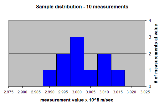
OK – Well we now have tried to get rid of as many error sources as possible, and we are confident we can measure the speed of light accurately to three significant figures.  (Maybe not enough for a trip on the space shuttle, but enough for an “A” in the class.)  We decide to make 10 measurements, and if they all agree, we are done.  We take 10 measurements, and we obtain the following distribution of measurement data.

• 1 measurement at          2.990 * 10⁸ m/sec
• 2 measurements at        2.995 * 10⁸ m/sec
• 3 measurements at        3.000 * 10⁸ m/sec
• 1 measurement at          3.005 * 10⁸ m/sec
• 2 measurements at        3.010 * 10⁸ m/sec
• 1 measurement at          3.015 * 10⁸ m/sec

Well they don’t agree, but they are all close to each other.  We decide to plot these values on a plot called a histogram (mainly because we want to impress the professor).  A histogram plots the number of times a particular measurement value occurs (actually the number of times it falls between two values) vs the actual value of the measurement.  Our histogram of the ten measurements looks like the following diagram.

Histogram of 10 data measurements shown above plotted on a graph - number of measurements at a value vs the values.

Using this histogram, we see the following: 

• First, from our measurements, we see that the speed of light is near 3 * 10⁸ meters/second.
• Second, the most probable value for the speed of light is 3.00 * 10⁸ meters/second.  Three of our measurements had this value, while the other values only had one or two measurements at those values.
• Third, the average value for the speed of light from these ten measurements is 3.002 * 10⁸ meters/sec.
• Finally, even through there is some uncertainty in our measurements, they are bracketed between 2.990 * 10⁸ and 3.015 * 10⁸ meters per second.  This eliminates a lot of values for the speed of light, so even though there is some uncertainty in our measurements, we have learned something about the speed of light.  I can say the speed of light is somewhere between 2.990 * 10⁸ and 3.015 * 10⁸ meters/sec.  We have an idea of the error bars of our experiment.  The true value for the speed of light probably falls somewhere between these two numbers.

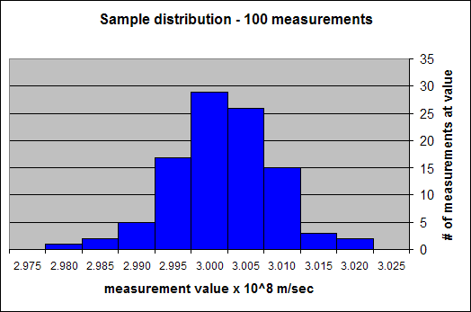
Since we are now having fun in our physics lab (a few of us geeks really do think physics is fun); since we are starting to understand a little bit about uncertainty in making measurements; and since we really need a “A+” in this lab to help us make up for a bad mid-term grade, we decide to take 100 measurements, and then draw a histogram of the results.  Our new histogram looks like:

Histogram of 100 data measurements plotted on a graph - number of measurements at a value vs the values. The histogram is starting to form a bell shape.

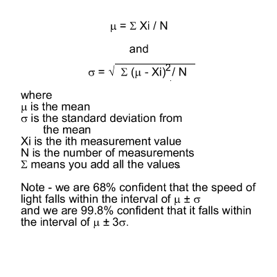
From this histogram, we see that again the most probable value for the speed of light is 3.000 * 10⁸ meters/sec, that the average (or mean) value is 3.0018*10⁸ meters/sec.  We also note that the average value is closer to the most probable value.  Someone in our group then remembers reading something about the standard deviation of a distribution, and says we should calculate that.  We calculate both the mean and the standard deviation as shown in the following diagram:

Mean and standard deviation calculations. The mean is found by adding up all the measurements, and then dividing by the number of measurements. The standard deviation is calculated by taking the difference between each of the data points and the mean, squaring them and adding them together, then dividing by the number of data points, and finally by taking the square root. The mean or average is an obvious quantity. We are all used to averaging sets of numbers. The standard deviation (sometimes called sigma (σ) for the Greek letter used to symbolize it) however is not as easy to understand. The standard deviation is a measure of how confident we are that the true speed of light is obtained from our set of measurements. We are about 68% confident that the true value of the speed of light falls between our mean minus one standard deviation and the mean plus one standard deviation (the mean plus or minus 1 standard deviation). We are also 99.8% confident that the true value for the speed of light falls within the mean value plus or minus three standard deviations. We have not determined the true speed of light absolutely, but we have bracketed the truth and we can state how confident we are that the truth falls within those brackets. We now have error bars for our faith in our value for the speed of light. We basically know how much confidence we can place in our value of the speed of light, and we can even associate a probability of being right (or wrong) to our value.

For our 100 measurements, we calculate the mean to be 3.0018 * 10⁸ meters/second, and the standard deviation to be 0.0072 * 10⁸ meters/second.  We aren’t sure what we are really doing, so we decide to look up the significance of the standard deviation.  We find out that the standard deviation is a value that allows us to have a level of confidence in our measurements.  In other words, we are about 68% sure that the true value for the speed of light will fall within the interval of the mean plus or minus the standard deviation, or between 2.9946 * 10⁸ meters/second and 3.0090 * 10⁸ meters/second.  We also read that we are 99.8% confident that the actual value of the speed of light falls somewhere in the interval of plus or minus three times the standard deviation around our mean value.  We are now at the point that we can know how much faith to put in our observations of the speed of light.  We have measured or quantified our doubt.

Suppose we really need some extra credit and therefore decide to automate our speed of light experiment so that we could make millions of measurements instead of just 10 or 100.  We would find our histograms would become a continuous function or a continuous probability distribution.

Gaussian distribution. When a large number of data points are collected, a probability distribution can be plotted (similar to the above histograms). Many times in a case like this, a bell shaped curve called a normal or Gaussian distribution results. Also shown on this chart are the mean (or average) value, μ, and the ±1 σ points and the ±3 σ points. 68% of the area under the curve falls between the ±1 σ points, and 99.8% of the area under the curve falls between the ±3 σ points. (Note - μ is the Greek letter mu used to represent the mean, and σ is the Greek letter sigma used to represent the standard deviation.)

This particular distribution is called a Gaussian distribution.  Not all probability distributions are this symmetric (I cheated a little on this one), but many of them are.  In this case, the mean is at the peak of the distribution (3.000 * 108 meters/second), and the standard deviation is 0.0071 * 108 meters/second.  (I won’t go into how I calculated it.)  On this graph I have shown where the ±1 σ (standard deviation) values, and the ±3 σ values fall on the graph.  Again my estimate of the speed of light (from the mean) and the error bars of my estimate are better than my measurements from either 100 or 10 measurements.

Adding other error sources. The mean and standard deviation values discussed above in many cases pertain to the statistical probability of making a measurement. Many times, we are making measurements at the limits of what our equipment can do. Other error sources like those discussed in the side box above would also need to be taken into account when we are trying to determine our true error bars or level of confidence. If all the error sources are independent of each other, then we would do this by squaring all the error sources including the statistical ones, adding them all together, and then taking the square root of this sum. This process is called root square summing or RSSing. This can be done both with standard deviations, in which case we get a new standard deviation, or it can be done using absolute uncertainties (three times the standard deviations) to get an absolute uncertainty (99.8% confidence).

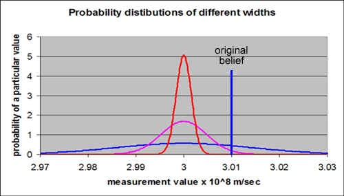
The more precisely we can make our measurements, the more faith we can put in the results of our measurements. Suppose we take even more pains to eliminate uncertainty sources in our experiments.   As we remove uncertainty, the probability distribution for our measurement of the speed of light becomes narrower.  This is illustrated in the following figure. If the red Gaussian resulted from our experiments, we would be more confident of our data then if either the violet or blue Gaussians resulted from our experiments. The error bars on our knowledge of the speed of light are smaller in the red Gaussian, so the error bars on our faith in the red Gaussian measurements are also smaller. The red Gaussian measurements are much closer to the truth than either the violet or the blue Gaussian measurements.

Various probability distributions. More precise measurements result in a narrower probability distribution. A narrower distribution means we have less uncertainty or narrower error bars on the faith we place in that measurement.

Another insight from this figure is that as we narrow the error bars on our knowledge, often we need to revise what we are placing our faith in. Suppose the vertical blue line at 3.01 * 10⁸ meters/second represents our original belief of the speed of light (the value we originally measured and had placed our faith in). When our knowledge had the error bars or uncertainty represented by the blue probability distribution, our original belief was a reasonable belief. But as we learned more and reduced the error bars on our knowledge, then our original belief was shown to be wrong, and we needed to revise what we were believing. For this value, our probability of being right went down and our probability of being wrong went up. If the red probability distribution represented our measurement, then we would be more than 99.99% confident that the speed of light is not 3.01 * 10⁸ meters/second. Instead we would believe that 3.00 * 10⁸ meters/second was a better value for the speed of light.

How does this discussion apply to the error bars on our religious faith?

So let’s revisit the questions I asked in the first paragraph:

• What are the error bars or limits of uncertainty on your faith?
• How confident are you in what you believe?
• Are you certain that what you believe is true?
• What is the probability that you believe something wrong?
• How would you quantify it?

The fact is, we all believe in many things – religiously, scientifically, politically, practically, …  On some things, the error bars on what we believe can be wide with very little consequence, but on the important things of life, we must focus on getting as close to the truth as possible.  If God exists and He is Who He says He is, then narrowing in on the truth about God is the most important pursuit we could be involved in, because our eternity is at stake.  Maybe we cannot completely eliminate the error bars on our knowledge of God and our faith.  But if God is God, I believe He would not leave us groping in the dark for the truth concerning Him, but instead He would have given us ample evidence for the truth about Him.  He would not expect us to trust in Him using just “blind faith.”  One of my purposes of this website is to explore and narrow in on the truth that we can know about God, and thereby narrow the error bars of our faith.

 

 

(next)
(back to index)